Anatoly Kondratenko - Probabilistic Theory of Stock Exchanges

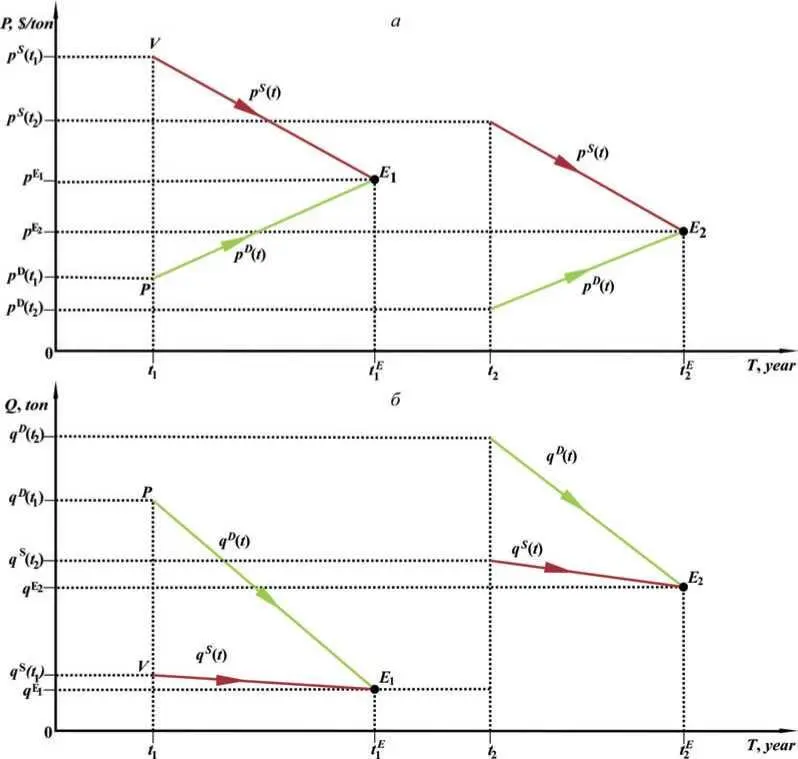
Fig. 1.3. Diagram of buyer and seller trajectories. The dynamics of the classical two-agent market economy in the economic space of price ( a ) and quantity ( b ) is depicted. Together, both parts of the figure represent the evolution of the economy over time in two-dimensional PQ -space.

This whole trading process, or simply bargaining, can be interpreted as a dynamic business exchange game between buyer and seller with the purpose of making a profit or achieving some other goal.

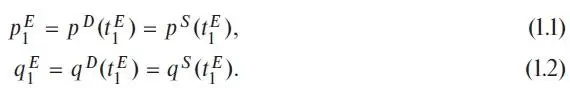
Let’s suppose that the negotiations went well and ended with the conclusion of a sale and purchase deal at time t 1 E . This means that at that moment in time the values of prices ( p D ( t ) and ( p S ( t )) and quantities ( q D ( t ) and ( q S(t )) in the quotations become equal, since obviously only specific mutually agreed price р 1 Е and quantity q 1 Е of goods can be specified in the contract. Let us assume that in this bargaining model it makes some sense to call these price and quantity values the market price and quantity of the commodity and to assume that the market itself comes to or reaches its equilibrium state at these price and quantity values. Formally, this is described using the following equations for the market price and quantity:

So, for the two-agent model we obtained this trivial but significant result: the very fact of reaching equilibrium makes it possible to conduct a transaction and maximize the volume of trades in monetary terms. In this simple case the conclusion is quite obvious: no agreement, no equilibrium, no transaction, trading volume is zero. But we will further show that this conclusion has a rather universal nature, which agrees with the postulated trade volume maximization principle. By the way, it is easy to show that in the framework of the neoclassical theory the maximum trade volume in natural terms, i.e. the maximum quantity of traded goods is reached at the equilibrium point.

Further on, since life does not stand still, the buyer and the seller can meet again and make new deals, but under new conditions and, obviously, with other prices and quantities, then for convenience we will call р 1 Е the first market price, and q 1 Е the first market quantity. Thus, at time t 1 E, the interests of the buyer and the seller have coincided for the first time, and they have been optimally satisfied by concluding a sale-purchase transaction. In this case agents, naturally, in the course of the market process (negotiations and changes in quotations) implicitly took into account the influence of the external environment and institutional factors on this and other markets, i.e. the economy as a whole. Here one can notice a similarity in the motion of the economic system in economic space, described by the trajectories of the buyer р D ( t ) and q D ( t ) and the seller р S ( t ) and q S ( t ), and in the motion of the two-particle physical system in real space, described by the trajectories of particles x 1(t ) и x 2(t ), which, by the way, are also the result of a certain physical maximization principle, namely, the principle of least action on the physical system.

The noted analogy with the physical system suggests using a similar mathematical body, analytical and graphical. In Fig. 1.3, to begin with, we provided a graphical representation of these trajectories of agents' motion as a time function using suitable coordinate systems time-price ( T, P ) and time-quantity ( T, Q ), similar to the construction of particle trajectories in classical mechanics. Please, note that figure 1.3 reflects a certain standard situation in the market, when buyer and seller intentionally meet at a point in time and start discussing a potential deal by mutual exchange of information about their conditions, first of all, desired prices and quantities of goods. During the negotiation, they continuously change their quotations until they agree to final terms on price р 1 Е and quantity q 1 Е at the time t 1 E. Such a simple «negotiation» market model is applicable, for example, to the economy of a fictional island on which, let us say for certainty, once a year there is a negotiated grain trade between a farmer and a hunter. To introduce some certainty, let us assume that they use the American dollar, $, for settlement. For clarity, in Fig. 1.3, as in the following figures, we use arrows to reflect the direction of agents’ movement during the market process.

So, in our classical negotiation model, up to the moment t 1 the market is in the simplest dormant state, there is no trade at all. At time t 1 , a buyer and a seller of grain appear in the market, and set their initial desired prices and quantity of grain: р D ( t 1 ), р S ( t 1 ) and q D ( t 1 ), q S ( t 1 ) points P and V in the graph show the position of the buyer and the seller at the initial moment of time t 1 when trade negotiations begin. Naturally, the desires of buyer and seller do not immediately coincide; the buyer wants a low price, but the seller is fighting for a higher price. However, both need to reach an understanding and subsequent deal, otherwise the farmer and the hunter will have a difficult next year. The negotiation process continues, with the market agents' process of changing their quotations reflecting its progress. As a result, the positions of the market agents converge, and they coincide at time t 1 E , which corresponds to the point of trajectories intersection Е 1 on the graphs.

On mutually beneficial terms at time t 1 E a voluntary transaction is performed. Then the market sinks back into a dormant state until the next harvest and the next year's sale at time t 2 .

Let’s assume, for certainty, that the new season's crop has increased, so q S(t 2)>q S(t 1) . In this case the seller obviously has to set the starting price lower right away, p S ( t 2 ) < p S ( t 1 ), while the buyer also takes the opportunity to lower the price and increase his amount of grain: p D ( t 2) < p D(t 1) and q D(t 2) > q D(t 1). In this case it is natural to expect that the trajectories of the buyer and the seller will be slightly different, and the agreement between the buyer and the seller will be reached with different parameters than in the previous bidding round.

Conditionally, we will describe the situation in the market at each moment of time using a set of real market prices and quantities of real transactions that actually take place in the market. As can be seen from Fig. 1.3, in our model real transactions occur in the market only at such moments of time as t 1 E and t 2 E when the following market equilibrium conditions are true (points in Fig. 1.3)

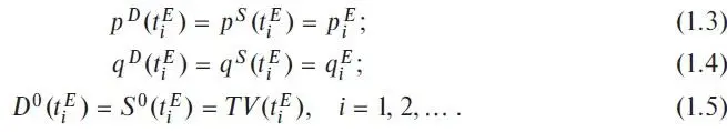
In formulas (1.3)-(1.5) we used several new concepts and definitions that require some explanation. We will explain it in some detail, as it is important for understanding the subsequent presentation of the theory. First, the concept of S&D plays one of the central roles in modern economic theory. The same applies to probabilistic economic theory, which, as we said above, can to some extent be interpreted as a theory of supply and demand. Intuitively, on a qualitative descriptive level, all economists understand what this concept means. Difficulties and discrepancies appear only in practice when trying to give a mathematical interpretation of these concepts and to develop an adequate method for their calculation and measurement. For this purpose, various theories containing different mathematical models of S&D have been developed. These theories use various S&D functions to formally define and quantify S&D.

In this paper we will also repeatedly provide various mathematical representations of this concept within the framework of probabilistic economics, complementing each other. For example, in the framework of our two-agent classical economics (negotiation model) let’s represent the S&D functions as follows:

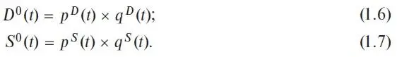
In equations (1.6) and (1.7), we have defined at each time t the total buyer demand function, D 0 ( t ) and the total seller supply function, S 0(t), as the multiplication of price and quantity quotations. For brevity, we shall hereafter refer to them simply as supply and demand functions, i.e., we shall omit the word «total» unless this could lead to confusion. These functions can easily be depicted in the time and S&D coordinate system, namely: [T, S&D], as shown in Fig. 1.4, which shows a diagram of the complete S&D functions. As expected, the S&D functions also intersect at the equilibrium point E 1 . More strictly, the equilibrium point is exactly the point in the diagram where the price and quantity quotations of the buyer and seller are equal. The fact that the S&D functions are also equal at this point is a simple consequence of their definition and the equality of prices and quantities in this point.

The last remark concerns the formula for estimating the market trade volume (Trade Volume, hereafter TV ) in the market TV ( t 1 E ) between a buyer and a seller at those moments in time when they come to a mutual understanding and conclude a transaction at an equilibrium point. Clearly, one can simply multiply the equilibrium values of price and quantity in this classical market model to obtain the trade turnover, or the total volume of all transactions, which follows from the above formula. The dimension of trade volume is the product of the dimensions of price and quantity; in our example, it is $. The same is true for the dimensions of the functions S&D, namely D 0 ( t ) и S 0 ( t ). Based on Fig. 1.4 we can conclude that it is at the equilibrium point that the trade volume reaches its maximum value. This result, which is self-evident and trivial in this case, is, in our opinion, rather general and principled: using it, we can deduce an assumption that markets tend to reach the equilibrium where maximum sales in monetary terms are achieved. It is possible to formulate this statement differently – in the form of the following hypothesis: markets strive for the maximum trading volume that is reached in equilibrium conditions, which agrees with the principle of trade volume maximization.

Fig. 1.4. Diagram of functions S&D, reflecting the dynamics of the classical two-agent market economy in the coordinate system [ T, S & D ] in the first time interval [ t 1,t 1 E ].